Descriptive Statistics for Data Science
This is the 3rd post of blog post series ‘Probability & Statistics for Data Science’, this post covers these topics related to descriptive statistics and their significance in data science.
- Introduction to Statistics
- Descriptive Statistics
- Uni-variate Analysis
- Bi-variate Analysis
- Multivariate Analysis
- Function Models
- Significance in Data Science
Visit ankitrathi.com now to:
— to read my blog posts on various topics of AI/ML
— to keep a tab on latest & relevant news/articles daily from AI/ML world
— to refer free & useful AI/ML resources
— to buy my books on discounted price
— to know more about me and what I am up to these days
Statistics Introduction
Statistics is a mathematical body of science that pertains to the collection, analysis, interpretation or explanation, and presentation of data.
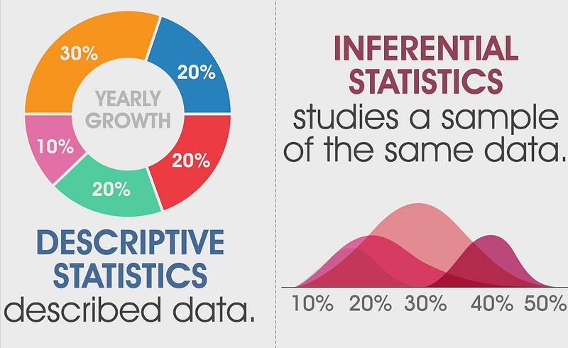
Statistics, in short, is the study of data. It includes descriptive statistics (the study of methods and tools for collecting data, and mathematical models to describe and interpret data) and inferential statistics (the systems and techniques for making probability-based decisions and accurate predictions.
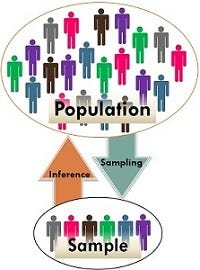
Population vs Sample
Population means the aggregate of all elements under study having one or more common characteristic while sample is a part of population chosen at random for participation in the study.
Descriptive Statistics
A descriptive statistic is a summary statistic that quantitatively describes or summarizes features of a collection of information. Descriptive statistics are just descriptive. They do not involve generalizing beyond the data at hand.
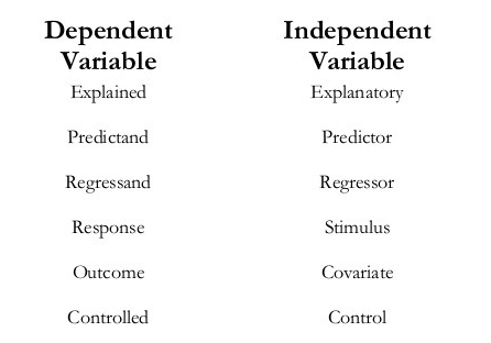
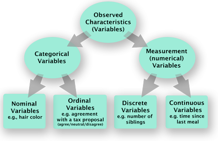
Types of Variable
Dependent and Independent Variables: An independent variable (experimental or predictor) is a variable that is being manipulated in an experiment in order to observe the effect on a dependent variable (outcome).
Categorical and Continuous Variables: Categorical variables (qualitative) represent types of data which may be divided into groups. Categorical variables can be further categorized as either nominal, ordinal or dichotomous. Continuous variables (quantitative) can take any value. Continuous variables can be further categorized as either interval or ratio variables.
Central Tendency
Central tendency is a central or typical value for a distribution.It may also be called a center or location of the distribution. The most common measures of central tendency are the arithmetic mean, the median and the mode.
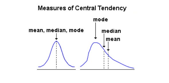
Mean is the numerical average of all values, median is directly in the
middle of the data set while mode is the most frequent value in the data set.
Spread or Variance
Spread (dispersion or variability) is the extent to which a distribution is stretched or squeezed. Common examples of measures of statistical dispersion are the variance, standard deviation, and inter-quartile range (IQR).
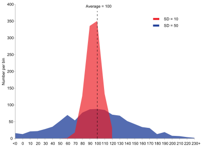
Inter-quartile range (IQR) is the distance between the 1st quartile and 3rd quartile and gives us the range of the middle 50% of our data. Variance is the average of the squared differences from the mean while standard deviation is the square root of the variance.
Upper outliers: Q3+1.5 ·IQR
Lower outliers: Q1–1.5 ·IQR
Standard Score or Z score: For an observed value x, the Z score finds the number of standard deviations x is away from the mean.
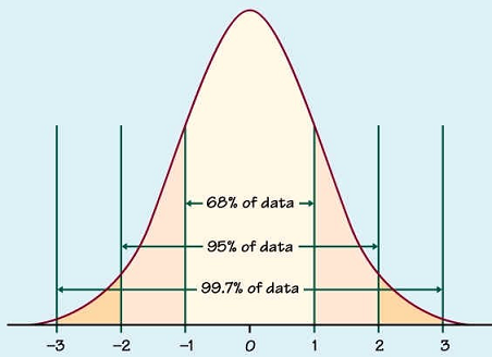
The Central Limit Theorem is used to help us understand the following facts regardless of whether the population distribution is normal or not:\
- the mean of the sample means is the same as the population mean\
- the standard deviation of the sample means is always equal to the standard error.\
- the distribution of sample means will become increasingly more normal as the sample size increases.
Uni-variate Analysis
In uni-variate analysis, appropriate statistic depends on the level of measurement. For nominal variables, a frequency table and a listing of the mode(s) is sufficient. For ordinal variables the median can be calculated as a measure of central tendency and the range (and variations of it) as a measure of dispersion. For interval level variables, the arithmetic mean (average) and standard deviation are added to the toolbox and, for ratio level variables, we add the geometric mean and harmonic mean as measures of central tendency and the coefficient of variation as a measure of dispersion.
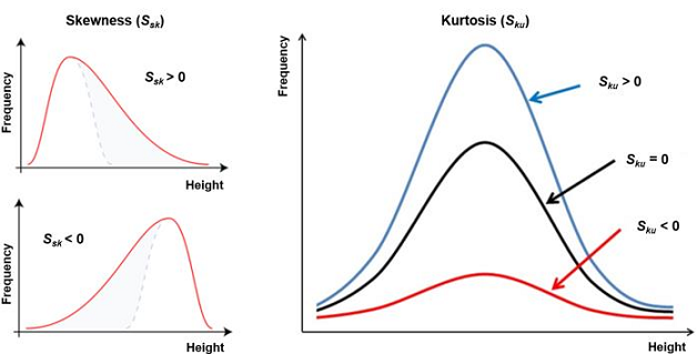
For interval and ratio level data, further descriptors include the variable’s skewness and kurtosis. Skewness is a measure of symmetry, or more precisely, the lack of symmetry. A distribution, or data set, is symmetric if it looks the same to the left and right of the center point. Kurtosis is a measure of whether the data are heavy-tailed or light-tailed relative to a normal distribution.
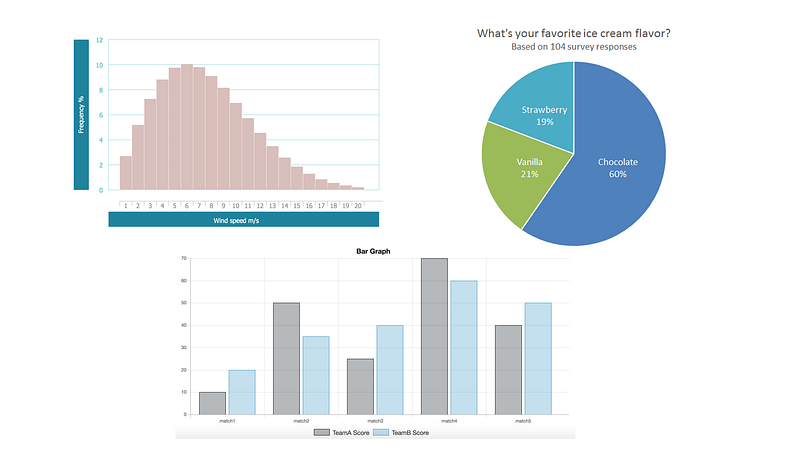
Mainly, bar graphs, pie charts and histograms are used for uni-variate analysis.
Bi-variate Distribution
Bivariate analysis involves the analysis of two variables (often denoted as X, Y), for the purpose of determining the empirical relationship between them.
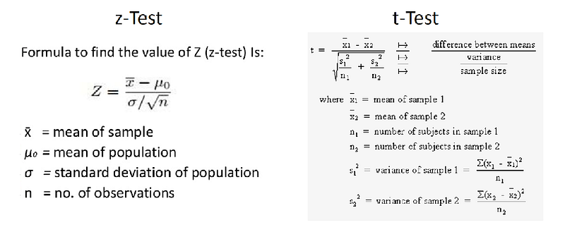
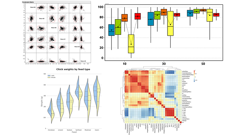
For two continuous variables, a scatter-plot is a common graph. When one variable is categorical and the other continuous, a box-plot or violin-plot (also Z-test and t-test) is common and when both are categorical a mosaic plot is common (also chi-square test).
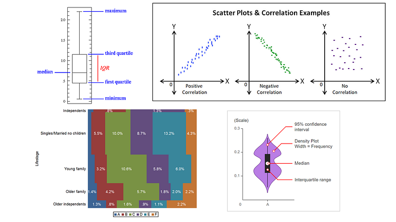
Multi-variate Analysis
Multi-variate analysis involves observation and analysis of more than one statistical outcome variable at a time. Multi-variate scatter plot, grouped box-plot (or grouped violin-plot), heat-map are used for multi-variate analysis.
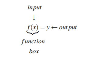
Function Models
A function can be expressed as an equation, as shown below. In the equation, f represents the function name and x represents the independent variable and y represents the dependent variable.
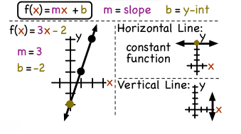
A linear function has the same average rate of change on every interval. When a linear model is used to describe data, it assumes a constant rate of change.
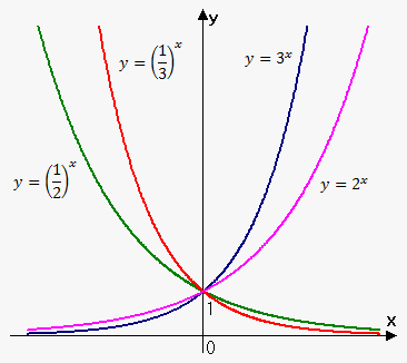
Exponential functions have variable appears as the exponent (or power) instead of the base.
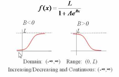
The logistic function has effect of limiting upper bound, a curve that grows exponentially at first and then slows down and hardly grows at all.
Significance in Data Science
Descriptive Statistics helps you to understand your data and is initial & very important step of Data Science. This is due to the fact that Data Science is all about making predictions and you can’t predict if you can’t understand the patterns in existing data.
References:
[embed]https://classroom.udacity.com/courses/ud827-india[/embed]
[embed]https://classroom.udacity.com/courses/ud827-india[/embed]
Ankit Rathi is an AI architect, published author & well-known speaker. His interest lies primarily in building end-to-end AI applications/products following best practices of Data Engineering and Architecture.
Why don’t you connect with Ankit on YouTube, Twitter, LinkedIn or Instagram?
If you have any questions or comments, click the "Go To Discussion" button below!